
Published on October 03, 2024
Table of Contents
 Image credit: DALL-E.
Your Autoscaling Journey So Far
Your company’s high-traffic SaaS product or e-commerce platform is humming along, and then—out of nowhere—traffic spikes. Your autoscaler is reacting, but it’s too slow to bring new nodes online, your app performance is tanking, and you notice your CTO has started typing to you in Slack… sh*t.
To your credit, the autoscaling solution you built with cluster-autoscaler or Karpenter works—just not fast enough. You’ve already fine-tuned the Horizontal Pod Autoscaler (HPA) configurations for CPU or memory, given yourself a generous “cushion” to absorb that initial traffic surge, and tweaked your application’s resource allocations to be true to their real usage and limits. But no matter how much you tweak, nothing seems to get around that minutes-long delay as your cloud provider brings new nodes online. Traffic just comes in too fast and furious.
Cue black-and-white infomercial scene: “There must be a better way!”
 Image credit: DALL-E.
Enter “Overprovisioning”
You’ve had a nice “chat” with your boss, and they’ve made it clear that they want this problem solved. Waiting for nodes to spin up after the fact just isn’t an option moving forward, as the business needs the complete trust of its customers to continue growing. These compute resources need to be ready in advance of any customer demand.
The approach to overprovisioning is pretty straightforward: you create low-priority pods using a PriorityClass that signals the autoscaler to bring nodes online before the workload arrives. These placeholder pods aren’t doing any actual work—they simply exist to ensure your infrastructure is prepped for when the real demand hits.
In practice, we’ll break this down into a three step process:
Step 1: Creating a PriorityClass resource: This is the key to marking these placeholder pods as low-priority, ensuring they’ll be preempted when higher-priority workloads come in.
Step 2: Deploying the overprovisioning pods: Using the PriorityClass, we’ll deploy placeholder pods that trigger the autoscaler to bring nodes online in advance of any actual demand.
Step 3: Determine your overprovisioning strategy: We’ll walk through different strategies for allocating resources of your overprovisioning pods, and choosing the best one depends on the needs of your workloads and traffic patterns.
Step 1: Create a PriorityClass Resource
apiVersion: scheduling.k8s.io/v1
kind: PriorityClass
metadata:
  name: overprovisioning
# Assigns a low priority to overprovisioning pods.
# Lower priority means they’re the first to be
# preempted when actual workloads need resources.
value: -10
globalDefault: false
description: "Priority class for overprovisioning to assist cluster-autoscaler"
The -10 priority value is crucial because it tells Kubernetes that these pods are low-priority placeholders. While the -10 value is arbitrary for this example, if there are other PriorityClass resources in the cluster, this number can be different. The most important thing here is that the value is low enough that our “overprovisioning” pods, which we will deploy in the next step, can be preempted by all of the real workloads. Due to the low PriorityClass, when real workloads are being scaled up in the cluster, the “overprovisioning” pods will then be evicted to make space, ensuring that your high-priority workloads get scheduled without any delay.
Step 2: Creating the Overprovisioning Deployment
Next, you’ll create the Deployment resource for your overprovisioning pods:
apiVersion: apps/v1
kind: Deployment
metadata:
  name: overprovisioning
spec:
  # Set the number of placeholder pods based
  # on how many nodes you want to bring online
  # in advance.
  replicas: 2
  selector:
    matchLabels:
      app: overprovisioning
  template:
    metadata:
      labels:
        app: overprovisioning
    spec:
      priorityClassName: overprovisioning # Link this pod to the overprovisioning PriorityClass we defined earlier.
      containers:
        - name: placeholder
          image: k8s.gcr.io/pause:3.1 # The 'pause' container is lightweight and ideal for placeholder pods.
          resources:
            requests:
              cpu: "XXXm" # Set based on your own workload requirements.
              memory: "XXXMi" # Same as above—customize based on your workload.
The replica count controls how many placeholder pods run. The value here will differ depending on the resource allocation strategy explained in the next section. Since these pods use PriorityClass with a -10 value, they’ll be evicted as soon as higher-priority workloads arrive, at which time new nodes will again be provisioned on which to schedule these lower priority pods, and the cycle repeats.
Step 3: Determining your Resource Allocation Strategy for Overprovisioning
There are a couple of different approaches to resource allocation for overprovisioning pods:
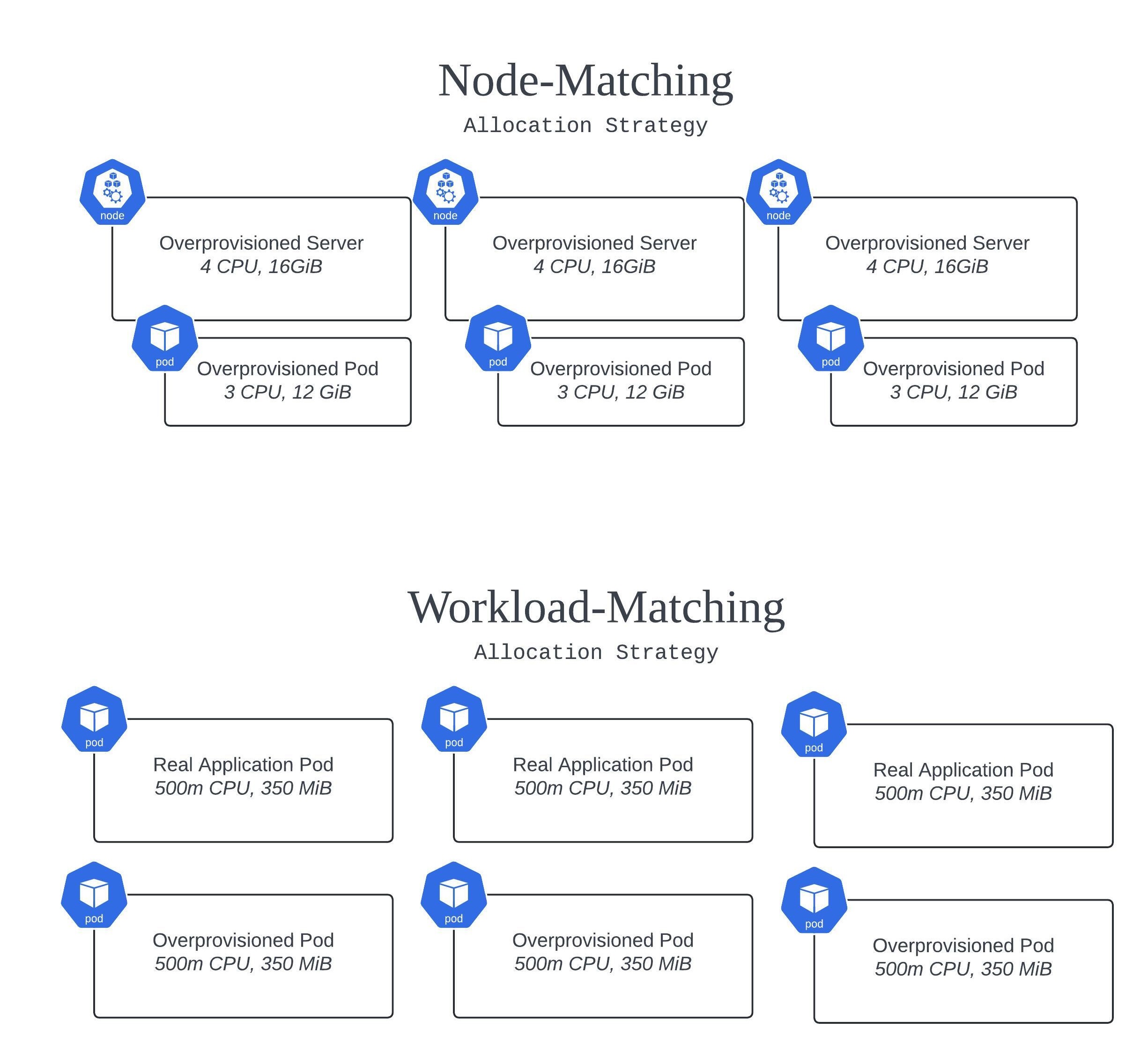
- Node-Matching: This approach ensures that each replica in your overprovisioning Deployment requests resources roughly equivalent to a full node’s capacity. For example, if your nodes have 4 CPU cores and 16 GiB of memory, you might set the CPU to 75% of that, leaving space for the kubelet and DaemonSets. This increases the chance that new nodes will be provisioned to accommodate each replica. In this scenario, you’ll have a 1:1 relationship between overprovisioning replicas and new nodes being brought online.
- Workload-Matching: If your goal is to scale up pods for a specific workload, match the resource requests of your overprovisioning pods to that workload. This allows you to scale quickly by “pre-reserving” resources for, say, 5 replicas of the actual workload. That pre-reservation may spin a new node or two online, or it may not depending on whether those 5 replicas can fit on existing nodes.
- Custom: You know your workloads better than anyone. If neither of the above strategies suits your needs, you can create your own allocation strategy tailored to your specific business and/or technical requirements.
Extending Basic Overprovisioning
Now that you’re overprovisioning your workloads, you’re watching those traffic spikes come in and breathing easy, for the most part. But nothing’s ever just that simple, is it?
Your boss comes over to you, mentioning they’re getting chewed out by the Chief Financial Officer for the sudden spike in server spend. While they can fend them off with the improved availability and reliability metrics your work has delivered, they’d still like you to take a look and see if there’s a way to optimize costs.
“No problem,” you reply. But as soon as you sit back down at your desk, another traffic spike hits—only this time, it’s bigger than ever before. Network traffic is surging, and you quickly realize the overprovisioning replicas you’ve set up aren’t going to be enough. Sure enough, customers are already seeing 500 Gateway Timeouts, and those Golden Signals are starting to lose their shine.
That muffin you put off eating earlier is going to have to wait a bit longer, now. It’s time to tackle these two problems, which you quickly deduce are somewhat related in the sense that some basic level of intelligence needs to be introduced, rather than blindly overprovisioning some no-op pods and hoping for the best.
On one hand, you’ve got predictable traffic spikes that are currently being handled just fine, but you need to optimize their costs. On the other hand, you have a marketing team that failed to inform your team about a coordinated campaign that’s suddenly bringing in thousands of new visitors to the site. Or maybe your company went viral (for better or for worse) due to a recent press release. Either way, you’ve got a sharp surge in unexpected visitors, something for which your system was only marginally designed to handle.
Optimizing the predictable, and handling the unpredictable. Time to earn that paycheck.
Optimizing the Predictable
As you dig into the nature of the workloads being scaled by the HPA, you notice something interesting: while the resource allocations for CPU and memory are accurately set for each workload, there’s still inefficiency in how nodes are being provisioned. For instance, your Payments service is a memory-heavy workload, using large amounts of RAM to cache transaction data, while your Auth service is CPU-intensive, needing significant CPU power for encryption and authentication processes.
The problem is that when new nodes come online, they’re not always the right type for the workload that’s being scheduled. For example, your Payments service, which requires a memory-optimized instance, might end up on a CPU-optimized node like an AWS c5.large or a Google Cloud C2 machine. On the flip side, your CPU-heavy Auth service might get scheduled onto a memory-optimized node like an AWS r5.large, Azure D-Family, or Google Cloud Z3 machine.
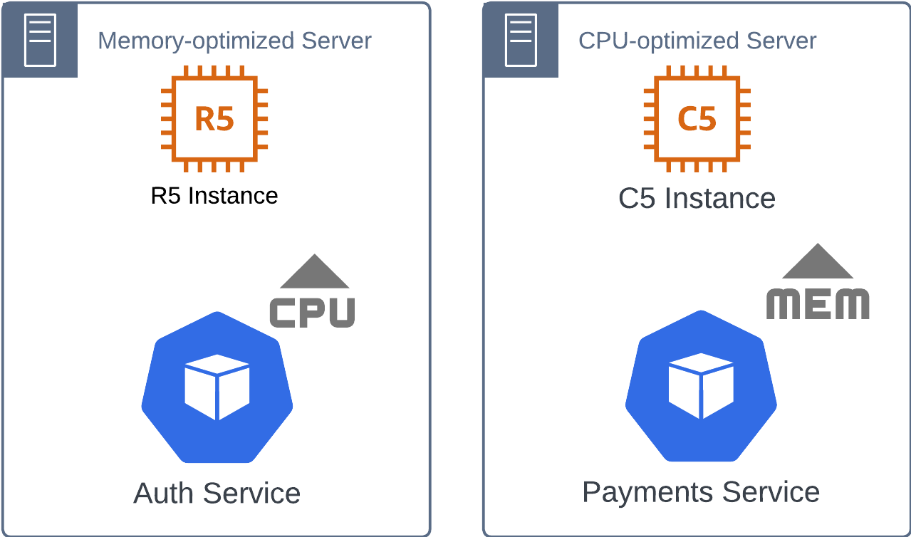
This mismatch between the workload’s resource demands and the node’s optimization means that, while the workloads are getting the resources they need, you’re paying for unused capacity—whether it’s idle CPU cores on a memory-optimized instance or extra memory that a CPU-heavy service doesn’t use. Over time, these inefficiencies start to add up and inflate your cloud bills.
The solution here is to ensure that each overprovisioning deployment is specifically tailored to the resource profile of the workload it’s intended to support. By matching CPU-heavy workloads to nodes optimized for CPU and memory-heavy workloads to nodes optimized for memory, you can make sure that when autoscaling kicks in, the workloads land on the right infrastructure. This reduces waste and optimizes costs.
You can achieve this by using taints, tolerations, and nodeSelectors to precisely match workloads to the right nodes. Let’s focus on implementing taints and tolerations, for now. Below are some examples for this exercise, followed by an explanation of how they work.
For example:
-
Taint your CPU-optimized nodes with
cpu-optimized=true:NoSchedule. -
Taint your memory-optimized nodes with
memory-optimized=true:NoSchedule.
Then, for your CPU-heavy Auth service, you add a toleration that allows it to be scheduled on the CPU-optimized nodes:
tolerations:
  - key: "cpu-optimized"
    operator: "Equal"
    value: "true"
    effect: "NoSchedule"
And for your memory-heavy Payments service, you add a toleration to allow it to be scheduled on the memory-optimized nodes:
tolerations:
  - key: "memory-optimized"
    operator: "Equal"
    value: "true"
    effect: "NoSchedule"
By using taints and tolerations, you’re effectively telling Kubernetes, “Allow CPU-heavy workloads to be scheduled on nodes optimized for CPU, and memory-heavy workloads on nodes optimized for memory.” In the example from earlier, pods from our Auth service would not have the toleration to be deployed to an overprovisioned memory-optimized node with their memory-optimized taint on it. This means that the resources on each node are being used more efficiently, but we can still do better at scheduling enforcement. It’s time to introduce nodeSelector into the mix.
While taints and tolerations control where a workload can be scheduled, nodeSelectors are used to make sure that a pod is scheduled on nodes with specific characteristics. For example, as we discussed earlier, you may want your CPU-heavy workloads to run exclusively on CPU-optimized nodes and your memory-heavy workloads to run exclusively on memory-optimized nodes.
For CPU-heavy pods, you could use a nodeSelector to ensure they’re only placed on nodes with the cpu-optimized label:
nodeSelector:
  node-type: "cpu-optimized"
Meanwhile, your memory-heavy pods can have a nodeSelector that ensures they’re scheduled on nodes labeled memory-optimized:
nodeSelector:
  node-type: "memory-optimized"
This gives you an additional level of control, so that workloads are not only allowed on certain nodes (using taints and tolerations), but are also actively scheduled on to the right kind of infrastructure.
By combining taints, tolerations, and nodeSelectors, you can fully control how and where your workloads are scheduled:
- Taint your nodes based on their optimization (e.g., CPU-optimized or memory-optimized).
- Add tolerations to your workloads to allow them to be scheduled on the appropriate nodes.
- Use nodeSelectors to enforce that your workloads are placed on nodes that match their resource profile.
This granular control gives you the ability to maintain workload efficiency on each server, avoiding wasted resources.
We can still do better. You know your traffic spikes come in on a routine basis, like clockwork—let’s say between 9:00 AM and 12:00 PM local time, hitting peak traffic around 10:30 AM. That means from 10:30 AM to 8:59 AM the next day, those fancy new overprovisioned servers are sitting there idle, with little expectation of being utilized. Bad news bears. This is a prime opportunity for further cost optimization. It’s time to get custom with our approach, with KEDA.
If you’re not familiar with KEDA yet, feel free to click the link above and check it out. It’s a Swiss Army knife for scaling workloads. KEDA gives you the capability to scale based on all kinds of custom or third-party parameters—like the length of a RabbitMQ queue, metrics from Prometheus, or a cron schedule, which is exactly what we need here. They support a ton of different scalers, I strongly recommend poking around the documentation and even sandboxing it yourself.
To handle these scheduled traffic spikes, we’re going to make use of the Cron scaler. This effectively means we can use a cron-like schedule on our overprovisioning deployment, minimizing resource use (and costs!) during off-hours. Importantly, instead of keeping replicas scaled up all the way up throughout peak traffic, we can begin to scale down once peak traffic has arrived, and our infrastructure is handling everything smoothly. Right before 9:00 AM, say at 8:45 AM, we’ll tell Kubernetes (via a new ScaledObject resource that KEDA installs as a Custom Resource Definition or CRD) to significantly increase the number of replicas on the overprovisioning deployment. And at 10:45 AM, we’ll dial it right back down again. In this example, we will scale down the replicas to 5, but this is a decision you and your team will have to make for yourselves (i.e. What makes sense as a minimal overprovision replica count?).
Let’s see what that looks like:
apiVersion: keda.sh/v1alpha1
kind: ScaledObject
metadata:
  name: overprovisioning-cron
spec:
  scaleTargetRef:
	kind: Deployment
	name: overprovisioning # Target your overprovisioning deployment
  minReplicaCount: 1
  maxReplicaCount: 20
  triggers:
  - type: cron
    metadata:
      timezone: "America/New_York" # Adjust to your local time zone
      start: "45 8 * * 1-5" # Scale up at 8:45 AM, Monday to Friday
        end: "45 10 * * 1-5" # Scale down at 10:45 AM, Monday to Friday
        desiredReplicas: "20" # Scale up to 20 replicas at 8:45 AM
  - type: cron
    metadata:
        timezone: "America/New_York"
        start: "45 10 * * 1-5" # Begin scaling down at 10:45 AM, Monday to Friday
        end: "45 8 * * 1-5" # Keep at least 5 replicas during off-peak hours
        desiredReplicas: "5" # Scale down to 5 replicas after traffic subsides
Here’s an explanation of the above code:
-
ScaledObject: This resource is installed by KEDA and enables you to define custom scaling behavior. In this case, we’re targeting the
overprovisioningdeployment. -
Cron Triggers:
- The first trigger starts at 8:45 AM and scales up the replicas to 20 to prepare for the expected traffic spike by 9:00 AM.
- The second trigger begins at 10:45 AM and scales the replicas back down to 5 after the traffic has hit its peak, and you no longer need overprovisioning servers for cushion.
-
Timezone: Make sure you adjust the
timezonefield to match your local time zone to ensure scaling happens at the right times, and don’t forget to take daylight savings time into account (if it applies).
So, at this point you’ve optimized the machine configurations that are launched, maximizing resource efficiency and thereby reducing the total number of servers you need to overprovision, and you’ve optimized the schedules of the overprovisioned machines themselves. This makes your CFO very happy. For now, at least.
Handling the Unpredictable
To tackle our second problem, we’re going to once again look at KEDA for a solution. This is a classic nail for our proverbial hammer, CPU-based autoscaling. You might think HPA, but let’s read this bit from KEDA’s FAQ page:
We recommend not to combine using KEDA’s
ScaledObjectwith a Horizontal Pod Autoscaler (HPA) to scale the same workload. They will compete with each other resulting given KEDA uses Horizontal Pod Autoscaler (HPA) under the hood and will result in odd scaling behavior. If you are using a Horizontal Pod Autoscaler (HPA) to scale on CPU and/or memory, we recommend using the CPU scaler & Memory scaler scalers instead.
We’ll use the CPU scaler in this example because we’re going to assume that the workloads that we want to scale up during unexpected traffic spikes are CPU bound, but you should certainly adjust which scaler is right for you.
In this scenario, we’re targeting our actual workloads rather than the overprovisioning deployment. This means we’ll need to create a new ScaledObject resource for these workloads to dynamically scale them based on CPU usage.
The new ScaledObject resource might look a little something like this:
apiVersion: keda.sh/v1alpha1
kind: ScaledObject
metadata:
  name: app-workload-cpu-scaler # Name of the ScaledObject for your workload
  namespace: default # Adjust this if your workload is in a different namespace
spec:
  scaleTargetRef:
    kind: Deployment
    name: app-deployment # The name of your actual application deployment
  minReplicaCount: 3 # Minimum replicas to keep running at all times
  maxReplicaCount: 15 # Maximum replicas to scale up to during CPU spikes
  triggers:
  - type: cpu
    metadata:
      type: "Utilization" # Scale based on CPU utilization
      value: "75" # Scale up when CPU usage exceeds 75%
Here’s an explanation of what you see above:
-
scaleTargetRef:
- This defines the workload we’re targeting for scaling. We’re targeting a Kubernetes deployment called
app-deployment, which represents an actual application or workload (not the overprovisioning pods).
- This defines the workload we’re targeting for scaling. We’re targeting a Kubernetes deployment called
-
minReplicaCount:
- This sets the minimum number of replicas that should always be running. Even if traffic is low or there’s no significant CPU activity, we want to ensure at least 3 replicas are available to handle the baseline traffic, and to maintain high availability.
-
maxReplicaCount:
- This defines the upper limit on scaling. In this case, we’ve set it to 15 replicas, which means during a significant traffic spike, KEDA will scale the deployment up to a maximum of 15 replicas.
-
CPU Trigger:
- The CPU scaler is being used in this example, with a 75% CPU utilization threshold. This means if the CPU usage for the deployment exceeds 75%, KEDA will automatically scale up the number of replicas to ensure the application can handle the increased load.
- If the CPU usage drops below 75%, KEDA will scale down the replicas accordingly, keeping things efficient.
This configuration allows KEDA to dynamically adjust your application’s replicas in real time based on actual CPU usage. If a sudden, unexpected traffic spike hits – whether it’s from a viral social media post, a surprise marketing campaign, or something else – the system will react immediately and scale the replicas to keep up with demand.
In this example, KEDA is effectively replacing the role of the HPA by using its CPU scaler to ensure your application can scale to handle unpredictable traffic spikes, all while maintaining cost efficiency by scaling down when the load decreases.
What We’ve Accomplished
Congratulations! You now have a robust, multi-situational, fully automated cloud scaling solution in place that keeps your infrastructure costs lean and mean, while handling every traffic load scenario under the sun. No such thing as a silver bullet, right? Well, you’ve come pretty close. By combining overprovisioning with KEDA’s Cron Scaler and metric-based scaling, you’ve not only handled predictable traffic but also prepared for the unpredictable. I’d say you’ve earned that muffin now.
Comparison to AWS EC2 Warm Pools
So, how does this approach stack up against AWS EC2 Warm Pools? Let’s take a look.
AWS EC2 Warm Pools are a feature that allows you to pre-provision EC2 instances and keep them in a “warm” state—meaning they’re initialized but not fully running, which drastically reduces the time it takes to bring them online. This is a great way to reduce startup time for EC2 instances that are expected to come under load, similar to how we handle overprovisioning in Kubernetes.
Similarity with Overprovisioning in Kubernetes
Minimizing Wait Time
Both EC2 Warm Pools and Kubernetes overprovisioning aim to minimize the time it takes to respond to a sudden surge in traffic. In both cases, you’re not waiting around for infrastructure to spin up in real-time—you’ve already got resources on standby.
Standby Capacity
Overprovisioning pods in Kubernetes act similarly to EC2 Warm Pools, in that they keep a portion of your system’s capacity “on deck” and ready to handle spikes when they arrive.
Key Differences
Node-Level vs. Instance-Level
The most obvious difference is that Warm Pools operate at the EC2 instance level, while overprovisioning in Kubernetes operates at the pod and node level. In Kubernetes, you’re dealing with fine-grained resource management, while EC2 Warm Pools are more about having entire virtual machines ready to go.
Scope and Flexibility
Overprovisioning in Kubernetes, especially with tools like Karpenter, allows you to scale based on very specific resource needs (like scaling memory-heavy workloads on memory-optimized nodes). EC2 Warm Pools, on the other hand, focus on full EC2 instances, so there’s less flexibility when it comes to resource-specific optimizations like CPU vs. memory.
Key Takeaways
Extending Autoscaling for Real-World Load Requirements
Whether you’re using cluster-autoscaler or Karpenter, the base functionality is great, but it doesn’t always cover all the nuances of real-world traffic. Extending your scaling with a pragmatic and cost-effective approach is critical.
Overprovisioning: A Starting Point, Not the Whole Solution
Overprovisioning on its own can be enough for some workloads, but it often needs a little extra boost. We’ve shown you how to go beyond basic overprovisioning by introducing KEDA to your cluster, bringing your system to the next level of responsiveness and efficiency.
Smart Scaling for Every Traffic Scenario
The key to handling both predictable and unpredictable traffic lies in being smart about scaling. By scheduling scaling for known traffic spikes and reacting dynamically to unexpected ones, you’ve covered your bases and ensured your infrastructure is always ready without the need to waste resources.
Acknowledgments
- Image of the Kubernetes wizard, and black and white infomercial style image of the SRE at his laptop pulling their hair out by DALL-E.